
Sub-pixel Distance Transform
High quality font rendering for WebGPU
This page includes diagrams in WebGPU, which has limited browser support. For the full experience, use Chrome on Windows or Mac, or a developer build on other platforms.
In this post I will describe Use.GPU's text rendering, which uses a bespoke approach to Signed Distance Fields (SDFs). This was borne out of necessity: while SDF text is pretty common on GPUs, some of the established practice on generating SDFs from masks is incorrect, and some libraries get it right only by accident. So this will be a deep dive from first principles, about the nuances of subpixels.

SDFs
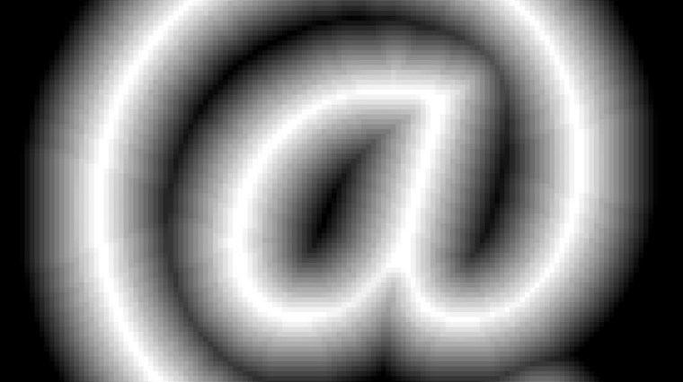
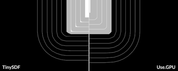
The idea behind SDFs is quite simple. To draw a crisp, anti-aliased shape at any size, you start from a field or image that records the distance to the shape's edge at every point, as a gradient. Lighter grays are inside, darker grays are outside. This can be a lower resolution than the target.

Then you increase the contrast until the gradient is exactly 1 pixel wide at the target size. You can sample it to get a perfectly anti-aliased opacity mask:
This works fine for text at typical sizes, and handles fractional shifts and scales perfectly with zero shimmering. It's also reasonably correct from a signal processing math point-of-view: it closely approximates averaging over a pixel-sized circular window, i.e. a low-pass convolution.
Crucially, it takes a rendered glyph as input, which means I can remain blissfully unaware of TrueType font specifics, and bezier rasterization, and just offload that to an existing library.
To generate an SDF, I started with MapBox's TinySDF library. Except, what comes out of it is wrong:
The contours are noticeably wobbly and pixelated. The only reason the glyph itself looks okay is because the errors around the zero-level are symmetrical and cancel out. If you try to dilate or contract the outline, which is supposed to be one of SDF's killer features, you get ugly gunk.
Compare to:
The original Valve paper glosses over this aspect and uses high resolution inputs (4k) for a highly downscaled result (64). That is not an option for me because it's too slow. But I did get it to work. As a result Use.GPU has a novel subpixel-accurate distance transform (ESDT), which even does emoji. It's a combination CPU/GPU approach, with the CPU generating SDFs and the GPU rendering them, including all the debug viz.
The Classic EDT
The common solution is a Euclidean Distance Transform. Given a binary mask, it will produce an unsigned distance field. This holds the squared distance d² for either the inside or outside area, which you can sqrt.


Like a Fourier Transform, you can apply it to 2D images by applying it horizontally on each row X, then vertically on each column Y (or vice versa). To make a signed distance field, you do this for both the inside and outside separately, and then combine the two as inside – outside or vice versa.
The algorithm is one of those clever bits of 80s-style C code which is O(N), has lots of 1-letter variable names, and is very CPU cache friendly. Often copy/pasted, but rarely understood. In TypeScript it looks like this, where array is modified in-place and f, v and z are temporary buffers up to 1 row/column long. The arguments offset and stride allow the code to be used in either the X or Y direction in a flattened 2D array.
for (let q = 1, k = 0, s = 0; q < length; q++) {
  f[q] = array[offset + q * stride];

  do {
    let r = v[k];
    s = (f[q] - f[r] + q * q - r * r) / (q - r) / 2;
  } while (s <= z[k] && --k > -1);

  k++;
  v[k] = q;
  z[k] = s;
  z[k + 1] = INF;
}

for (let q = 0, k = 0; q < length; q++) {
  while (z[k + 1] < q) k++;
  let r = v[k];
  let d = q - r;
  array[offset + q * stride] = f[r] + d * d;
}
To explain what this code does, let's start with a naive version instead.
Given a 1D input array of zeroes (filled), with an area masked out with infinity (empty):
O = [·, ·, ·, 0, 0, 0, 0, 0, ·, 0, 0, 0, ·, ·, ·]Make a matching sequence … 3 2 1 0 1 2 3 … for each element, centering the 0 at each index:
[0, 1, 2, 3, 4, 5, 6, 7, 8, 9,10,11,12,13,14] + ∞
[1, 0, 1, 2, 3, 4, 5, 6, 7, 8, 9,10,11,12,13] + ∞
[2, 1, 0, 1, 2, 3, 4, 5, 6, 7, 8, 9,10,11,12] + ∞
[3, 2, 1, 0, 1, 2, 3, 4, 5, 6, 7, 8, 9,10,11] + 0
[4, 3, 2, 1, 0, 1, 2, 3, 4, 5, 6, 7, 8, 9,10] + 0
[5, 4, 3, 2, 1, 0, 1, 2, 3, 4, 5, 6, 7, 8, 9] + 0
[6, 5, 4, 3, 2, 1, 0, 1, 2, 3, 4, 5, 6, 7, 8] + 0
[7, 6, 5, 4, 3, 2, 1, 0, 1, 2, 3, 4, 5, 6, 7] + 0
[8, 7, 6, 5, 4, 3, 2, 1, 0, 1, 2, 3, 4, 5, 6] + ∞
[9, 8, 7, 6, 5, 4, 3, 2, 1, 0, 1, 2, 3, 4, 5] + 0
[10,9, 8, 7, 6, 5, 4, 3, 2, 1, 0, 1, 2, 3, 4] + 0
[11,10,9, 8, 7, 6, 5, 4, 3, 2, 1, 0, 1, 2, 3] + 0
[12,11,10,9, 8, 7, 6, 5, 4, 3, 2, 1, 0, 1, 2] + ∞
[13,12,11,10,9, 8, 7, 6, 5, 4, 3, 2, 1, 0, 1] + ∞
[14,13,12,11,10,9, 8, 7, 6, 5, 4, 3, 2, 1, 0] + ∞
You then add the value from the array to each element in the row:
[∞, ∞, ∞, ∞, ∞, ∞, ∞, ∞, ∞, ∞, ∞, ∞, ∞, ∞, ∞]
[∞, ∞, ∞, ∞, ∞, ∞, ∞, ∞, ∞, ∞, ∞, ∞, ∞, ∞, ∞]
[∞, ∞, ∞, ∞, ∞, ∞, ∞, ∞, ∞, ∞, ∞, ∞, ∞, ∞, ∞]
[3, 2, 1, 0, 1, 2, 3, 4, 5, 6, 7, 8, 9,10,11]
[4, 3, 2, 1, 0, 1, 2, 3, 4, 5, 6, 7, 8, 9,10]
[5, 4, 3, 2, 1, 0, 1, 2, 3, 4, 5, 6, 7, 8, 9]
[6, 5, 4, 3, 2, 1, 0, 1, 2, 3, 4, 5, 6, 7, 8]
[7, 6, 5, 4, 3, 2, 1, 0, 1, 2, 3, 4, 5, 6, 7]
[∞, ∞, ∞, ∞, ∞, ∞, ∞, ∞, ∞, ∞, ∞, ∞, ∞, ∞, ∞]
[9, 8, 7, 6, 5, 4, 3, 2, 1, 0, 1, 2, 3, 4, 5]
[10,9, 8, 7, 6, 5, 4, 3, 2, 1, 0, 1, 2, 3, 4]
[11,10,9, 8, 7, 6, 5, 4, 3, 2, 1, 0, 1, 2, 3]
[∞, ∞, ∞, ∞, ∞, ∞, ∞, ∞, ∞, ∞, ∞, ∞, ∞, ∞, ∞]
[∞, ∞, ∞, ∞, ∞, ∞, ∞, ∞, ∞, ∞, ∞, ∞, ∞, ∞, ∞]
[∞, ∞, ∞, ∞, ∞, ∞, ∞, ∞, ∞, ∞, ∞, ∞, ∞, ∞, ∞]
And then take the minimum of each column:
P = [3, 2, 1, 0, 0, 0, 0, 0, 1, 0, 0, 0, 1, 2, 3]This sequence counts up inside the masked out area, away from the zeroes. This is the positive distance field P.
You can do the same for the inverted mask:
I = [0, 0, 0, ·, ·, ·, ·, ·, 0, ·, ·, ·, 0, 0, 0]to get the complementary area, i.e. the negative distance field N:
N = [0, 0, 0, 1, 2, 3, 2, 1, 0, 1, 2, 1, 0, 0, 0]That's what the EDT does, except it uses square distance … 9 4 1 0 1 4 9 …:
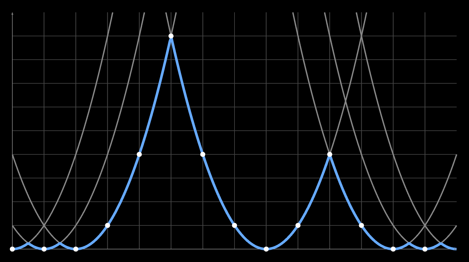
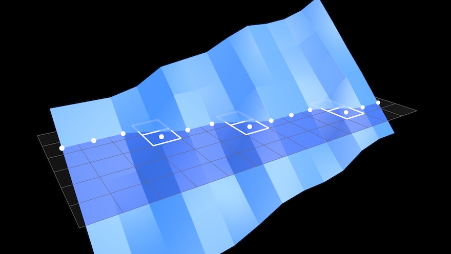
When you apply it a second time in the second dimension, these outputs are the new input, i.e. values other than 0 or ∞. It still works because of Pythagoras' rule: d² = x² + y². This wouldn't be true if it used linear distance instead. The net effect is that you end up intersecting a series of parabolas, somewhat like a 1D slice of a Voronoi diagram:
I' = [0, 0, 1, 4, 9, 4, 4, 4, 1, 1, 4, 9, 4, 9, 9]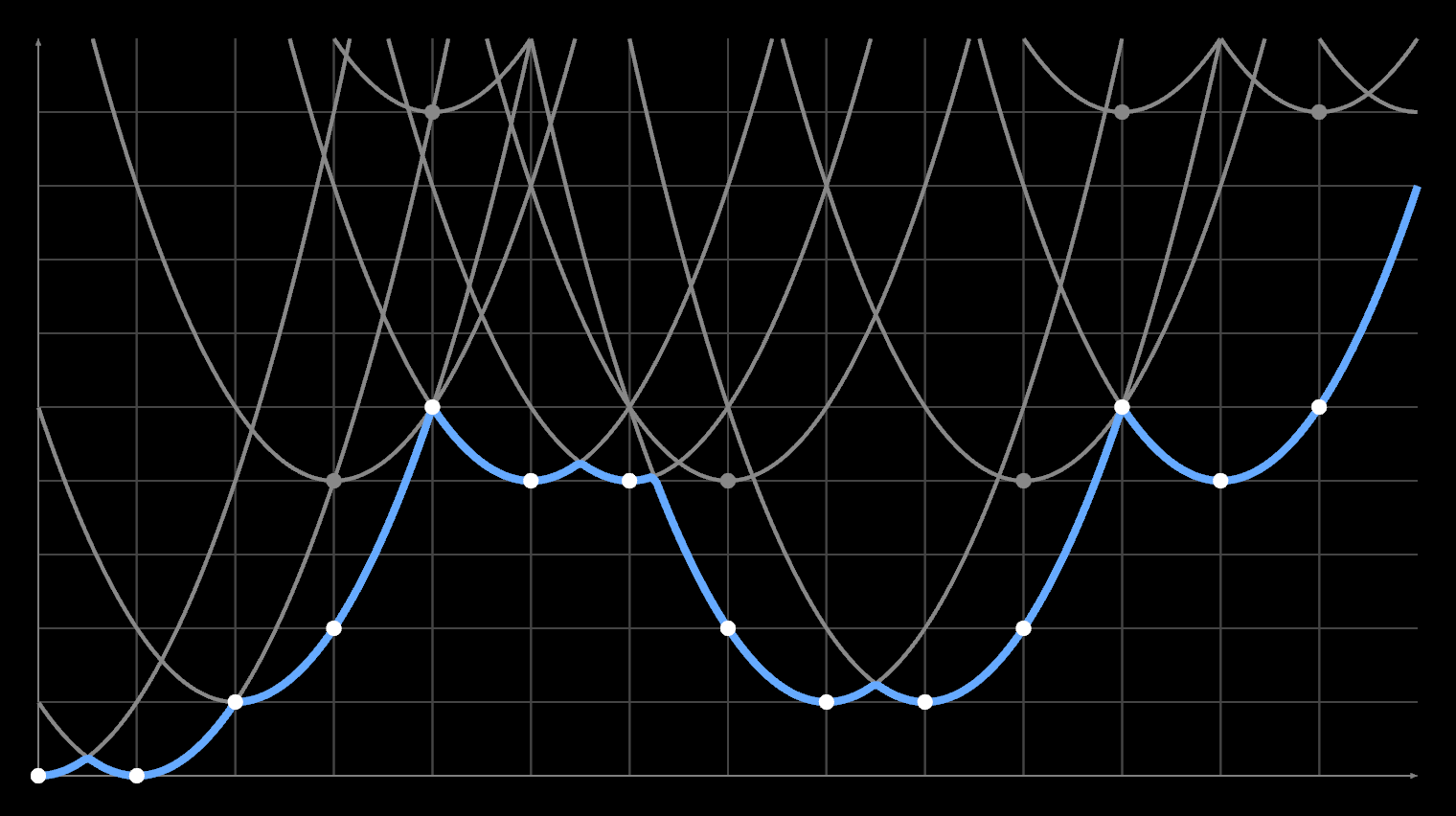
Each parabola sitting above zero is the 'shadow' of a zero-level paraboloid located some distance in a perpendicular dimension:
The code is just a more clever way to do that, without generating the entire N² grid per row/column. It instead scans through the array left to right, building up a list v[k] of significant minima, with thresholds s[k] where two parabolas intersect. It adds them as candidates (k++) and discards them (--k) if they are eclipsed by a newer value. This is the first for/while loop:
for (let q = 1, k = 0, s = 0; q < length; q++) {
  f[q] = array[offset + q * stride];

  do {
    let r = v[k];
    s = (f[q] - f[r] + q * q - r * r) / (q - r) / 2;
  } while (s <= z[k] && --k > -1);

  k++;
  v[k] = q;
  z[k] = s;
  z[k + 1] = INF;
}
Then it goes left to right again (for), and fills out the values, skipping ahead to the right minimum (k++). This is the squared distance from the current index q to the nearest minimum r, plus the minimum's value f[r] itself. The paper has more details:
for (let q = 0, k = 0; q < length; q++) {
  while (z[k + 1] < q) k++;
  let r = v[k];
  let d = q - r;
  array[offset + q * stride] = f[r] + d * d;
}
The Broken EDT
So what's the catch? The above assumes a binary mask.
As it happens, if you try to subtract a binary N from P, you have an off-by-one error:
    O = [·, ·, ·, 0, 0, 0, 0, 0, ·, 0, 0, 0, ·, ·, ·]
    I = [0, 0, 0, ·, ·, ·, ·, ·, 0, ·, ·, ·, 0, 0, 0]

    P = [3, 2, 1, 0, 0, 0, 0, 0, 1, 0, 0, 0, 1, 2, 3]
    N = [0, 0, 0, 1, 2, 3, 2, 1, 0, 1, 2, 1, 0, 0, 0]

P - N = [3, 2, 1,-1,-2,-3,-2,-1, 1,-1,-2,-1, 1, 2, 3]
It goes directly from 1 to -1 and back. You could add +/- 0.5 to fix that.
But if there is a gray pixel in between each white and black, which we classify as both inside (0) and outside (0), it seems to work out just fine:
    O = [·, ·, ·, 0, 0, 0, 0, 0, ·, 0, 0, 0, ·, ·, ·]
    I = [0, 0, 0, 0, ·, ·, ·, 0, 0, 0, ·, 0, 0, 0, 0]

    P = [3, 2, 1, 0, 0, 0, 0, 0, 1, 0, 0, 0, 1, 2, 3]
    N = [0, 0, 0, 0, 1, 2, 1, 0, 0, 0, 1, 0, 0, 0, 0]

P - N = [3, 2, 1, 0,-1,-2,-1, 0, 1, 0,-1, 0, 1, 2, 3]
This is a realization that somebody must've had, and they reasoned on: "The above is correct for a 50% opaque pixel, where the edge between inside and outside falls exactly in the middle of a pixel."
"Lighter grays are more inside, and darker grays are more outside. So all we need to do is treat l = level - 0.5 as a signed distance, and use l² for the initial inside or outside value for gray pixels. This will cause either the positive or negative distance field to shift by a subpixel amount l. And then the EDT will propagate this in both X and Y directions."
The initial idea is correct, because this is just running SDF rendering in reverse. A gray pixel in an opacity mask is what you get when you contrast adjust an SDF and do not blow it out into pure black or white. The information inside the gray pixels is "correct", up to rounding.
But there are two mistakes here.
The first is that even in an anti-aliased image, you can have white pixels right next to black ones. Especially with fonts, which are pixel-hinted. So the SDF is wrong there, because it goes directly from -1 to 1. This causes the contours to double up, e.g. around this bottom edge:
To solve this, you can eliminate the crisp case by deliberately making those edges very dark or light gray.
But the second mistake is more subtle. The EDT works in 2D because you can feed the output of X in as the input of Y. But that means that any non-zero input to X represents another dimension Z, separate from X and Y. The resulting squared distance will be x² + y² + z². This is a 3D distance, not 2D.
If an edge is shifted by 0.5 pixels in X, you would expect a 1D SDF like:
  […, 0.5, 1.5, 2.5, 3.5, …]
= […, 0.5, 1 + 0.5, 2 + 0.5, 3 + 0.5, …]
Instead, because of the squaring + square root, you will get:
  […, 0.5, 1.12, 2.06, 3.04, …]
= […, sqrt(0.25), sqrt(1 + 0.25), sqrt(4 + 0.25), sqrt(9 + 0.25), …]
The effect of l² = 0.25 rapidly diminishes as you get away from the edge, and is significantly wrong even just one pixel over.
The correct shift would need to be folded into (x + …)² + (y + …)² and depends on the direction. e.g. If an edge is shifted horizontally, it ought to be (x + l)² + y², which means there is a term of 2*x*l missing. If the shift is vertical, it's 2*y*l instead. This is also a signed value, not positive/unsigned.
Given all this, it's a miracle this worked at all. The only reason this isn't more visible in the final glyph is because the positive and negative fields contains the same but opposite errors around their respective gray pixels.
The Not-Subpixel EDT
As mentioned before, the EDT algorithm is essentially making a 1D Voronoi diagram every time. It finds the distance to the nearest minimum for every array index. But there is no reason for those minima themselves to lie at integer offsets, because the second for loop effectively resamples the data.
So you can take an input mask, and tag each index with a horizontal offset Δ:
O = [·, ·, ·, 0, 0, 0, 0, 0, ·, ·, ·]
Δ = [A, B, C, D, E, F, G, H, I, J, K]
As long as the offsets are small, no two indices will swap order, and the code still works. You then build the Voronoi diagram out of the shifted parabolas, but sample the result at unshifted indices.
Problem 1 - Opposing Shifts
This lead me down the first rabbit hole, which was an attempt to make the EDT subpixel capable without losing its appealing simplicity. I started by investigating the nuances of subpixel EDT in 1D. This was a bit of a mirage, because most real problems only pop up in 2D. Though there was one important insight here.
O = [·, ·, ·, 0, 0, 0, 0, 0, ·, ·, ·]
Δ = [·, ·, ·, A, ·, ·, ·, B, ·, ·, ·]
Given a mask of zeroes and infinities, you can only shift the first and last point of each segment. Infinities don't do anything, while middle zeroes should remain zero.
Using an offset A works sort of as expected: this will increase or decrease the values filled in by a fractional pixel, calculating a squared distance (d + A)² where A can be positive or negative. But the value at the shifted index itself is always (0 + A)² (positive). This means it is always outside, regardless of whether it is moving left or right.
If A is moving left (–), the point is inside, and the (unsigned) distance should be 0. At B the situation is reversed: the distance should be 0 if B is moving right (+). It might seem like this is annoying but fixable, because the zeroes can be filled in by the opposite signed field. But this is only looking at the binary 1D case, where there are only zeroes and infinities.
In 2D, a second pass has non-zero distances, so every index can be shifted:
O = [a, b, c, d, e, f, g, h, i, j, k]
Δ = [A, B, C, D, E, F, G, H, I, J, K]
Now, resolving every subpixel unambiguously is harder than you might think:
It's important to notice that the function being sampled by an EDT is not actually smooth: it is the minimum of a discrete set of parabolas, which cross at an angle. The square root of the output only produces a smooth linear gradient because it samples each parabola at integer offsets. Each center only shifts upward by the square of an integer in every pass, so the crossings are predictable. You never sample the 'wrong' side of (d + ...)². A subpixel EDT does not have this luxury.
Subpixel EDTs are not irreparably broken though. Rather, they are only valid if they cause the unsigned distance field to increase, i.e. if they dilate the empty space. This is a problem: any shift that dilates the positive field contracts the negative, and vice versa.
To fix this, you need to get out of the handwaving stage and actually understand P and N as continuous 2D fields.
Problem 2 - Diagonals
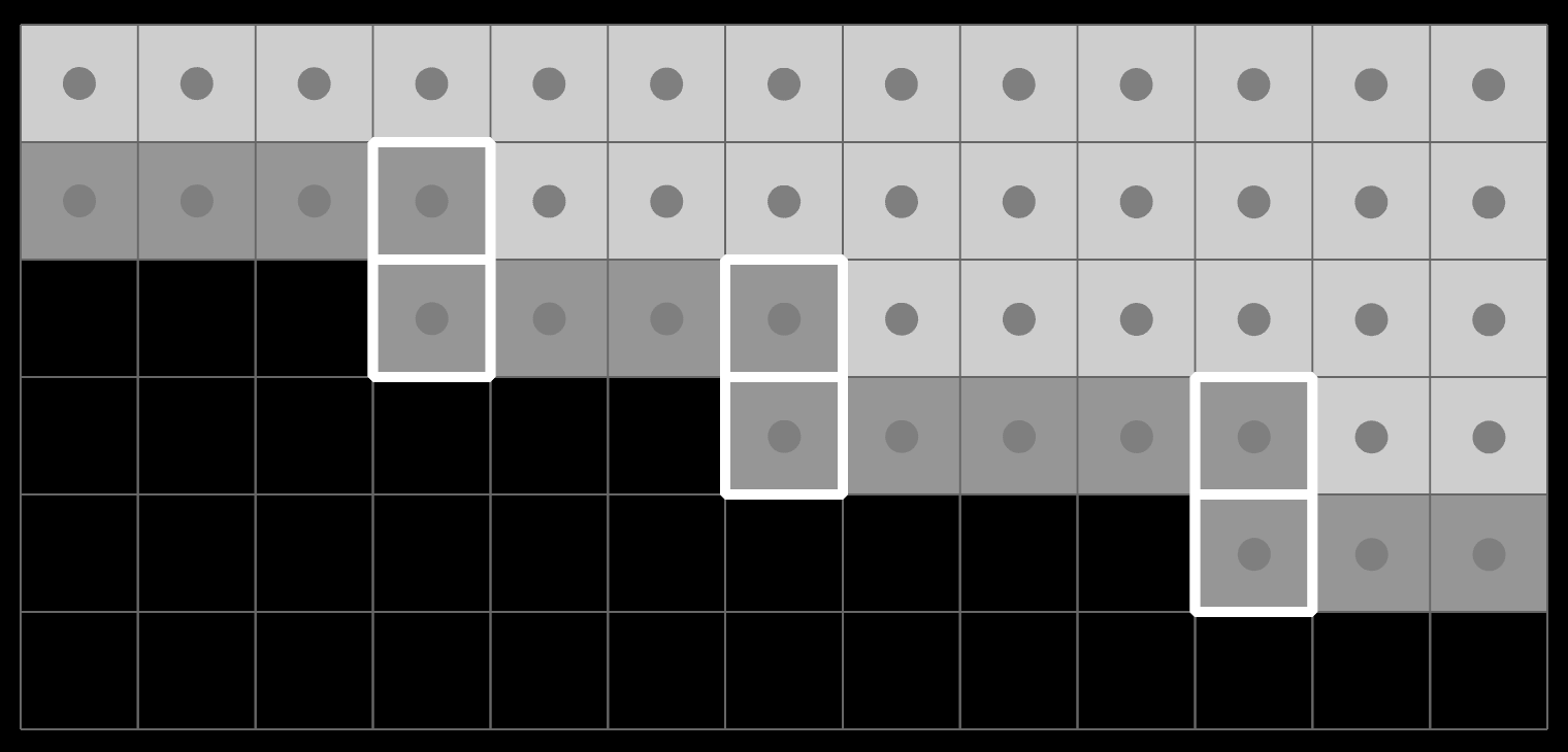
Consider an aliased, sloped edge. To understand how the classic EDT resolves it, we can turn it into a voronoi diagram for all the white pixel centers:
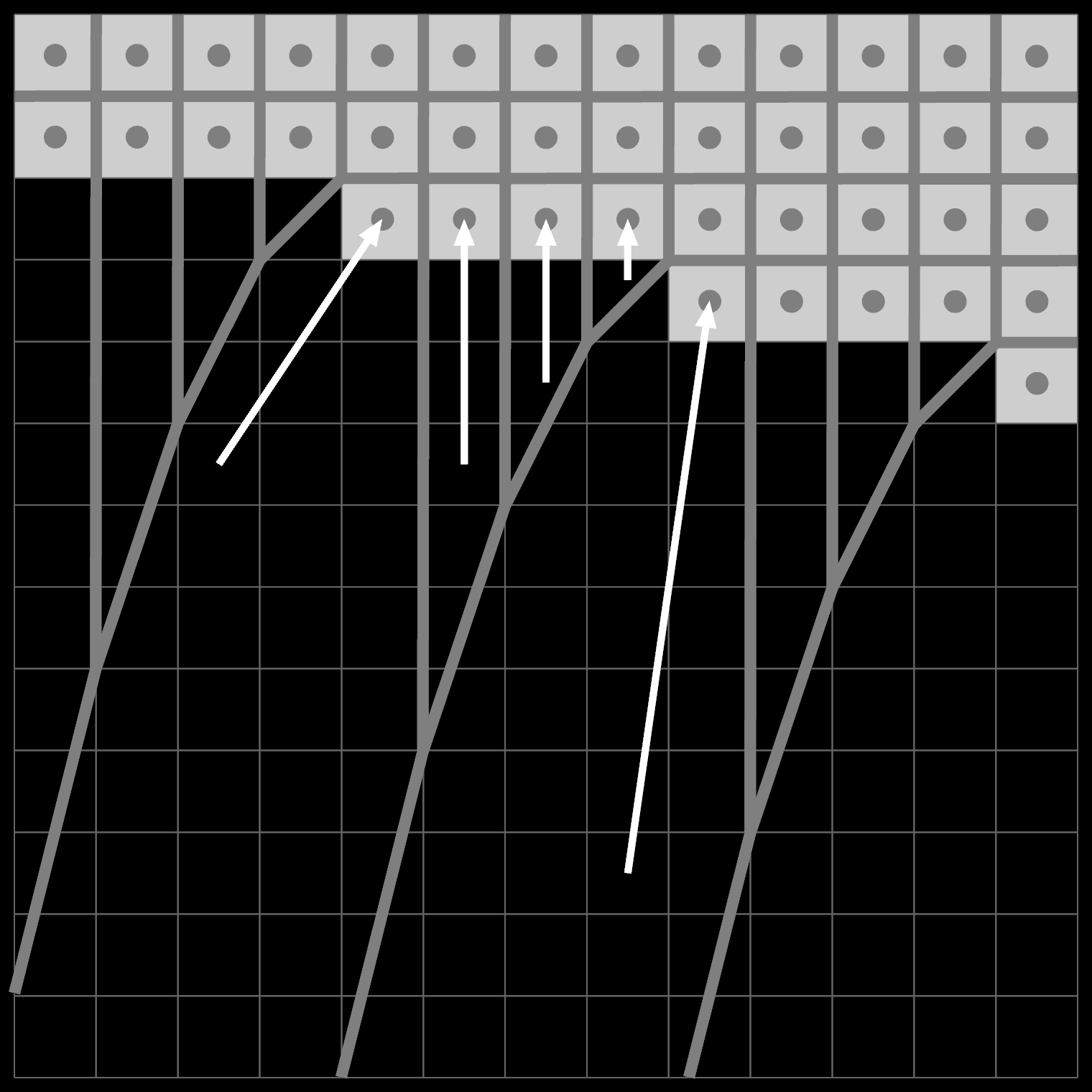
Near the bottom, the field is dominated by the white pixels on the corners: they form diagonal sections downwards. Near the edge itself, the field runs perfectly vertical inside a roughly triangular section. In both cases, an arrow pointing back towards the cell center is only vaguely perpendicular to the true diagonal edge.
Near perfect diagonals, the edge distances are just wrong. The distance of edge pixels goes up or right (1), rather than the more logical diagonal 0.707…. The true closest point on the edge is not part of the grid.
These fields don't really resolve properly until 6-7 pixels out. You could hide these flaws with e.g. an 8x downscale, but that's 64x more pixels. Either way, you shouldn't expect perfect numerical accuracy from an EDT. Just because it's mathematically separable doesn't mean it's particularly good.
In fact, it's only separable because it isn't very good at all.
Problem 3 - Gradients
In 2D, there is also only one correct answer to the gray case. Consider a diagonal edge, anti-aliased:
Thresholding it into black, grey or white, you get:
If you now classify the grays as both inside and outside, then the highlighted pixels will be part of both masks. Both the positive and negative field will be exactly zero there, and so will the SDF (P - N):
This creates a phantom vertical edge that pushes apart P and N, and causes the average slope to be less than 45º. The field simply has the wrong shape, because gray pixels can be surrounded by other gray pixels.
This also explains why TinySDF magically seemed to work despite being so pixelized. The l² gray correction fills in exactly the gaps in the bad (P - N) field where it is zero, and it interpolates towards a symmetrically wrong P and N field on each side.
If we instead classify grays as neither inside nor outside, then P and N overlap in the boundary, and it is possible to resolve them into a coherent SDF with a clean 45 degree slope, if you do it right:
What seemed like an off-by-one error is actually the right approach in 2D or higher. The subpixel SDF will then be a modified version of this field, where the P and N sides are changed in lock-step to remain mutually consistent.
Though we will get there in a roundabout way.
Problem 4 - Commuting
It's worth pointing out: a subpixel EDT simply cannot commute in 2D.
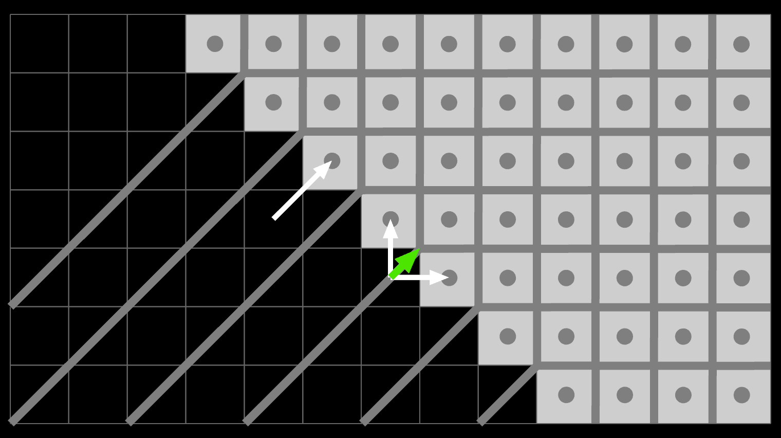
First, consider the data flow of an ordinary EDT:
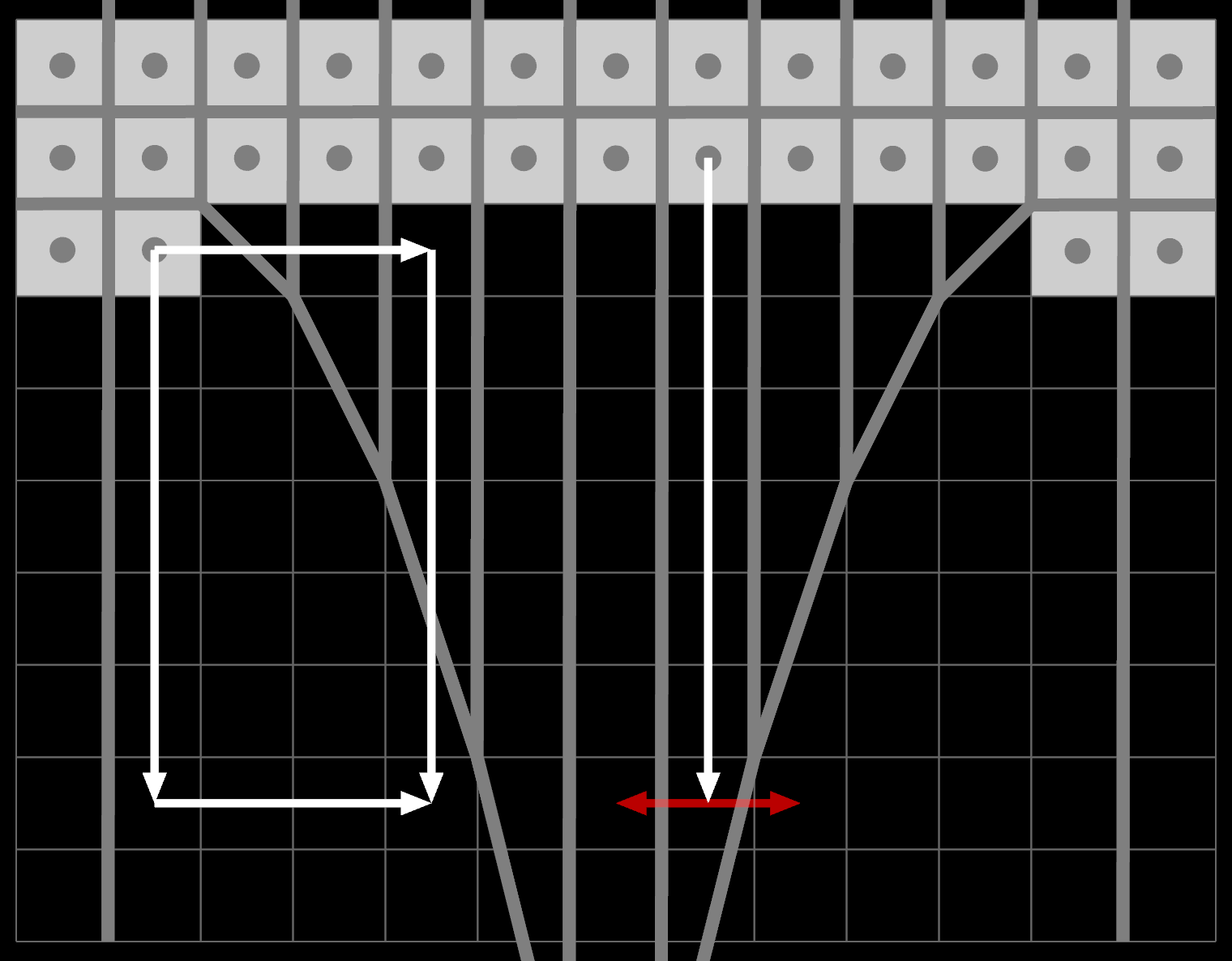
Information from a corner pixel can flow through empty space both when doing X-then-Y and Y-then-X. But information from the horizontal edge pixels can only flow vertically then horizontally. This is okay because the separating lines between adjacent pixels are purely vertical too: the red arrows never 'win'.
But if you introduce subpixel shifts, the separating lines can turn:
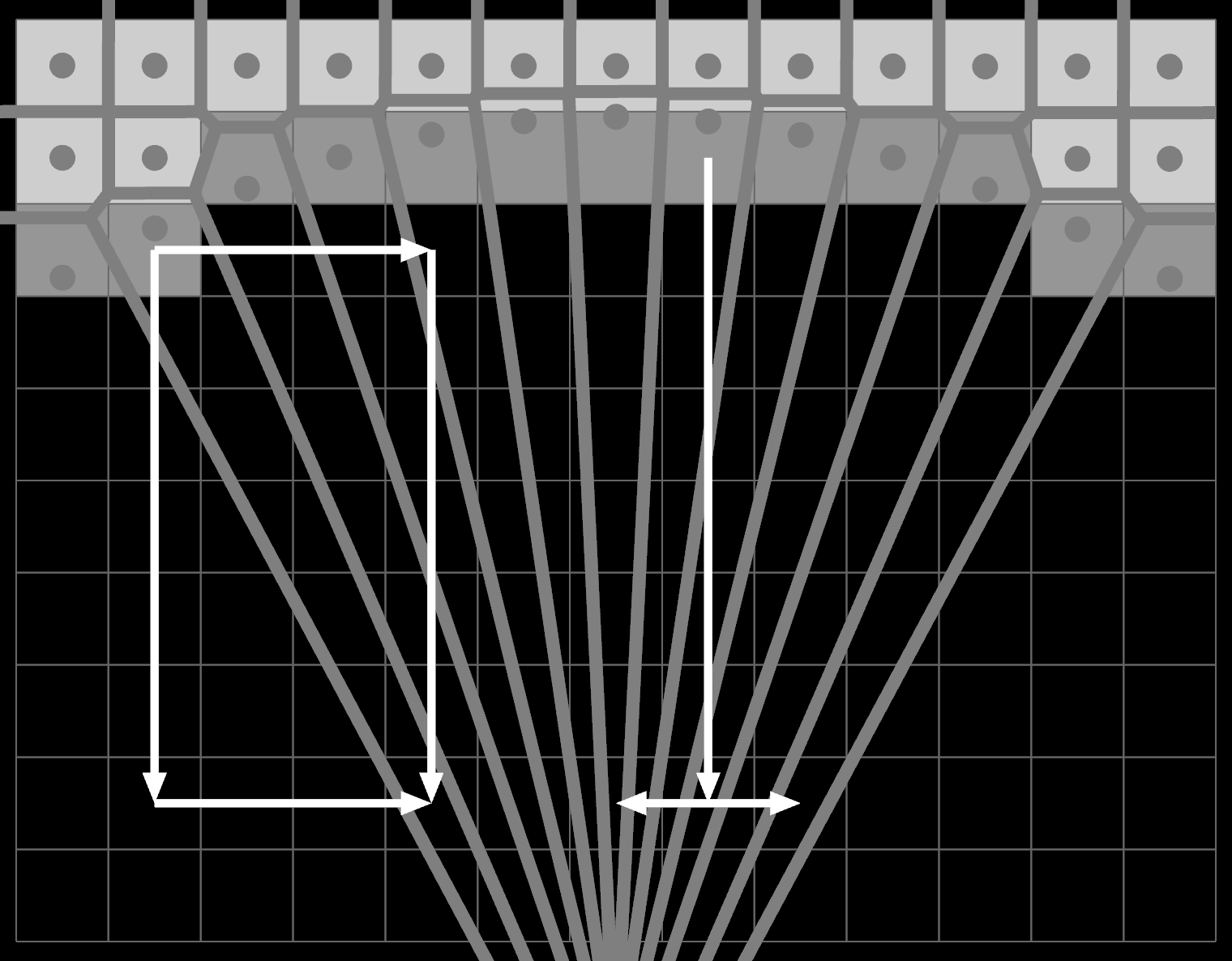
The data flow is still limited to the original EDT pattern, so the edge pixels at the top can only propagate by starting downward. They can only influence adjacent columns if the order is Y-then-X. For vertical edges it's the opposite.
That said, this is only a problem on shallow concave curves, where there aren't any corner pixels nearby. The error is that it 'snaps' to the wrong edge point, but only when it is already several pixels away from the edge. In that case, the smaller x² term is dwarfed by the much larger y² term, so the absolute error is small after sqrt.
The ESDT
Knowing all this, here's how I assembled a "true" Euclidean Subpixel Distance Transform.
Subpixel offsets
To start we need to determine the subpixel offsets. We can still treat level - 0.5 as the signed distance for any gray pixel, and ignore all white and black for now.
The tricky part is determining the exact direction of that distance. As an approximation, we can examine the 3x3 neighborhood around each gray pixel and do a least-squares fit of a plane. As long as there is at least one white and one black pixel in this neighborhood, we get a vector pointing towards where the actual edge is. In practice I apply some horizontal/vertical smoothing here using a simple [1 2 1] kernel.
The result is numerically very stable, because the originally rasterized image is visually consistent.
This logic is disabled for thin creases and spikes, where it doesn't work. Such points are treated as fully masked out, so that neighboring distances propagate there instead. This is needed e.g. for the pointy negative space of a W to come out right.
I also implemented a relaxation step that will smooth neighboring vectors if they point in similar directions. However, the effect is quite minimal, and it rounds very sharp corners, so I ended up disabling it by default.
The goal is then to do an ESDT that uses these shifted positions for the minima, to get a subpixel accurate distance field.
P and N junction
We saw earlier that only non-masked pixels can have offsets that influence the output (#1). We only have offsets for gray pixels, yet we concluded that gray pixels should be masked out, to form a connected SDF with the right shape (#3). This can't work.
SDFs are both the problem and the solution here. Dilating and contracting SDFs is easy: add or subtract a constant. So you can expand both P and N fields ahead of time geometrically, and then undo it numerically. This is done by pushing their respective gray pixel centers in opposite directions, by half a pixel, on top of the originally calculated offset:
This way, they can remain masked in in both fields, but are always pushed between 0 and 1 pixel inwards. The distance between the P and N gray pixel offsets is always exactly 1, so the non-zero overlap between P and N is guaranteed to be exactly 1 pixel wide everywhere. It's a perfect join anywhere we sample it, because the line between the two ends crosses through a pixel center.
When we then calculate the final SDF, we do the opposite, shifting each by half a pixel and trimming it off with a max:
SDF = max(0, P - 0.5) - max(0, N - 0.5)
Only one of P or N will be > 0.5 at a time, so this is exact.
To deal with pure black/white edges, I treat any black neighbor of a white pixel (horizontal or vertical only) as gray with a 0.5 pixel offset (before P/N dilation). No actual blurring needs to happen, and the result is numerically exact minus epsilon, which is nice.
ESDT state
The state for the ESDT then consists of remembering a signed X and Y offset for every pixel, rather than the squared distance. These are factored into the distance and threshold calculations, separated into its proper parallel and orthogonal components, i.e. X/Y or Y/X. Unlike an EDT, each X or Y pass has to be aware of both axes. But the algorithm is mostly unchanged otherwise, here X-then-Y.
The X pass:
At the start, only gray pixels have offsets and they are all in the range -1…1 (exclusive). With each pass of ESDT, a winning minima's offsets propagate to its affecting range, tracking the total distance (Δx, Δy) (> 1). At the end, each pixel's offset points to the nearest edge, so the squared distance can be derived as Δx² + Δy².
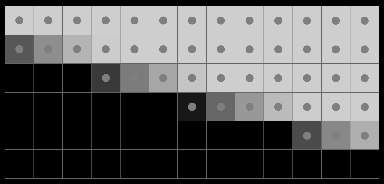
The Y pass:
You can see that the vertical distances in the top-left are practically vertical, and not oriented perpendicular to the contour on average: they have not had a chance to propagate horizontally. But they do factor in the vertical subpixel offset, and this is the dominant component. So even without correction it still creates a smooth SDF with a surprisingly small error.
Fix ups
The commutativity errors are all biased positively, meaning we get an upper bound of the true distance field.
You could take the min of X then Y and Y then X. This would re-use all the same prep and would restore rotation-independence at the cost of 2x as many ESDTs. You could try X then Y then X at 1.5x cost with some hacks. But neither would improve diagonal areas, which were still busted in the original EDT.
Instead I implemented an additional relaxation pass. It visits every pixel's target, and double checks whether one of the 4 immediate neighbors (with subpixel offset) isn't a better solution:
It's a good heuristic because if the target is >1px off there is either a viable commutative propagation path, or you're so far away the error is negligible. It fixes up the diagonals, creating tidy lines when the resolution allows for it:
You could take this even further, given that you know the offsets are supposed to be perpendicular to the glyph contour. You could add reprojection with a few dot products here, but getting it to not misfire on edge cases would be tricky.
While you can tell the unrelaxed offsets are wrong when visualized, and the fixed ones are better, the visual difference in the output glyphs is tiny. You need to blow glyphs up to enormous size to see the difference side by side. So it too is disabled by default. The diagonals in the original EDT were wrong too and you could barely tell.
Emoji
An emoji is generally stored as a full color transparent PNG or SVG. The ESDT can be applied directly to its opacity mask to get an SDF, so no problem there.


There are an extremely rare handful of emoji with semi-transparent areas, but you can get away with making those solid. For this I just use a filter that detects '+' shaped arrangements of pixels that have (almost) the same transparency level. Then I dilate those by 3x3 to get the average transparency level in each area. Then I divide by it to only keep the anti-aliased edges transparent.
The real issue is blending the colors at the edges, when the emoji is being rendered and scaled. The RGB color of transparent pixels is undefined, so whatever values are there will blend into the surrounding pixels, e.g. creating a subtle black halo:

Not Premultiplied

Premultiplied
A common solution is premultiplied alpha. The opacity is baked into the RGB channels as (R * A, G * A, B * A, A), and transparent areas must be fully transparent black. This allows you to use a premultiplied blend mode where the RGB channels are added directly without further scaling, to cancel out the error.
But the alpha channel of an SDF glyph is dynamic, and is independent of the colors, so it cannot be premultiplied. We need valid color values even for the fully transparent areas, so that up- or downscaling is still clean.
Luckily the ESDT calculates X and Y offsets which point from each pixel directly to the nearest edge. We can use them to propagate the colors outward in a single pass, filling in the entire background. It doesn't need to be very accurate, so no filtering is required.
RGB channel

Output
The result looks pretty great. At normal sizes, the crisp edge hides the fact that the interior is somewhat blurry. Emoji fonts are supported via the underlying ab_glyph library, but are too big for the web (10MB+). So you can just load .PNGs on demand instead, at whatever resolution you need. Hooking it up to the 2D canvas to render native system emoji is left as an exercise for the reader.
Use.GPU does not support complex Unicode scripts or RTL text yet—both are a can of worms I wish to offload too—but it does support composite emoji like "pirate flag" (white flag + skull and crossbones) or "male astronaut" (astronaut + man) when formatted using the usual Zero-Width Joiners (U+200D) or modifiers.
Shading
Finally, a note on how to actually render with SDFs, which is more nuanced than you might think.
I pack all the SDF glyphs into an atlas on-demand, the same I use elsewhere in Use.GPU. This has a custom layout algorithm that doesn't backtrack, optimized for filling out a layout at run-time with pieces of a similar size. Glyphs are rasterized at 1.5x their normal font size, after rounding up to the nearest power of two. The extra 50% ensures small fonts on low-DPI displays still use a higher quality SDF, while high-DPI displays just upscale that SDF without noticeable quality loss. The rounding ensures similar font sizes reuse the same SDFs. You can also override the detail independent of font size.
To determine the contrast factor to draw an SDF, you generally use screen-space derivatives. There are good and bad ways of doing this. Your goal is to get a ratio of SDF pixels to screen pixels, so the best thing to do is give the GPU the coordinates of the SDF texture pixels, and ask it to calculate the difference for that between neighboring screen pixels. This works for surfaces in 3D at an angle too. Bad ways of doing this will instead work off relative texture coordinates, and introduce additional scaling factors based on the view or atlas size, when they are all just supposed to cancel out.
As you then adjust the contrast of an SDF to render it, it's important to do so around the zero-level. The glyph's ideal vector shape should not expand or contract as you scale it. Like TinySDF, I use 75% gray as the zero level, so that more SDF range is allocated to the outside than the inside, as dilating glyphs is much more common than contraction.
At the same time, a pixel whose center sits exactly on the zero level edge is actually half inside, half outside, i.e. 50% opaque. So, after scaling the SDF, you need to add 0.5 to the value to get the correct opacity for a blend. This gives you a mathematically accurate font rendering that approximates convolution with a pixel-sized circle or box.
But I go further. Fonts were not invented for screens, they were designed for paper, with ink that bleeds. Certain renderers, e.g. MacOS, replicate this effect. The physical bleed distance is relatively constant, so the larger the font, the smaller the effect of the bleed proportionally. I got the best results with a 0.25 pixel bleed at 32px or more. For smaller sizes, it tapers off linearly. When you zoom out blocks of text, they get subtly fatter instead of thinning out, and this is actually a great effect when viewing document thumbnails, where lines of text become a solid mass at the point where the SDF resolution fails anyway.

In Use.GPU I prefer to use gamma correct, linear RGB color, even for 2D. What surprised me the most is just how unquestionably superior this looks. Text looks rock solid and readable even at small sizes on low-DPI. Because the SDF scales, there is no true font hinting, but it really doesn't need it, it would just be a nice extra.
Presumably you could track hinted points or edges inside SDF glyphs and then do a dynamic distortion somehow, but this is an order of magnitude more complex than what it is doing now, which is splat a contrasted texture on screen. It does have snapping you can turn on, which avoids jiggling of individual letters. But if you turn it off, you get smooth subpixel everything:
I was always a big fan of the 3x1 subpixel rendering used on color LCDs (i.e. ClearType and the like), and I was sad when it was phased out due to the popularity of high-DPI displays. But it turns out the 3x res only offered marginal benefits... the real improvement was always that it had a custom gamma correct blend mode, which is a thing a lot of people still get wrong. Even without RGB subpixels, gamma correct AA looks great. Converting the entire desktop to Linear RGB is also not going to happen in our lifetime, but I really want it more now.
The "blurry text" that some people associate with anti-aliasing is usually just text blended with the wrong gamma curve, and without an appropriate bleed for the font in question.
* * *
If you want to make SDFs from existing input data, subpixel accuracy is crucial. Without it, fully crisp strokes actually become uneven, diagonals can look bumpy, and you cannot make clean dilated outlines or shadows. If you use an EDT, you have to start from a high resolution source and then downscale away all the errors near the edges. But if you use an ESDT, you can upscale even emoji PNGs with decent results.
It might seem pretty obvious in hindsight, but there is a massive difference between getting it sort of working, and actually getting all the details right. There were many false starts and dead ends, because subpixel accuracy also means one bad pixel ruins it.
In some circles, SDF text is an old party trick by now... but a solid and reliable implementation is still a fair amount of work, with very little to go off for the harder parts.
By the way, I did see if I could use voronoi techniques directly, but in terms of computation it is much more involved. Pretty tho:
The ESDT is fast enough to use at run-time, and the implementation is available as a stand-alone import for drop-in use.
This post started as a single live WebGPU diagram, which you can play around with. The source code for all the diagrams is available too.